Materialize Formalism

Materialize is a system that maintains views over changing data.

At Materialize's heart are time-varying collections (TVCs). These are multisets of typed data whose contents may vary arbitrarily as function of some ordered time. Materialize records, transforms, and presents the contents of time varying collections.

Materialize's primary function is to provide the contents of time-varying collection at specific times with absolute certainty.

This document details the intended behavior of the system. It does not intend to describe the current behavior of the system. Various liberties are taken in the names of commands and types, in the interest of simplicity. Not all commands here may be found in the implementation, nor all implementation commands found here.

You may wish to consult the VLDB and CIDR papers on differential dataflow, as well as the DD library.

In a nutshell

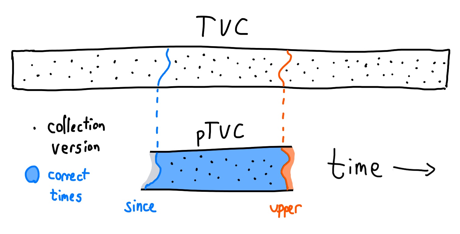
A time-varying collections (TVC) is a map of partially ordered times to collection versions, where each collection version is a multiset of typed pieces of data. Because the past and future of a TVC may be unknown, Materialize represents a TVC as a partial TVC (pTVC), which is an accurate representation of a TVC during a range of times bounded by two frontiers: a lower frontier since, and an upper frontier upper.

To avoid storing and processing the entire collection version for every single time, Materialize uses sets of updates as a differential representation of a pTVC. These updates are triples of [data, time, diff]: the piece of data being changed, the time of the change, and the change in multiplicity of that data. Materialize can compact a pTVC by merging updates from the past, and append new updates to a pTVC as they arrive. Compaction advances the since frontier of the pTVC, and appending advances the upper frontier. Both compact and append preserve correctness: these differential representations of a pTVC are faithful to the "real" TVC between since and upper.

Materialize identifies each TVC by a unique GlobalId, and maintains a mutable map of GlobalIds to the current pTVC representing that GlobalID's TVC.

Internally, Materialize is separated into three layers: storage, compute, and adapter. The storage layer records updates from (e.g.) external data sources. The compute layer provides materialized views: new TVCs which are derived from other TVCs in some way. The ability to write and read to these layers is given by a first-class capability object, which constrains when pTVCs can be compacted and appended to.

Users issue SQL queries to Materialize, but the storage and compute layers are defined in terms of low-level operations on update triples. The adapter translates these SQL queries into low-level commands. Since SQL does not (generally) include an explicit model of time, the adapter picks timestamps for SQL statements using a stateful timeline object. To map table names to GlobalIds and capabilities, Materialize maintains a source mapping. SQL indices are maintained by the compute layer.

Finally: Materialize's adapter supports SQL transactions.

In depth

Data

The term piece of data, in this document, means a single, opaque piece of arbitrary typed data. For example, one might use a piece of data to represent a single row in an SQL database, or a single key-value pair in a key-value store.

In this document, we often denote a piece of data as data. However, we want to emphasize that as far as updates are concerned, each piece of data is an opaque, atomic object rather than a composite type. When we describe an update to a row, that data includes the entire new row, not just the columns inside it which changed.

We say "piece of data" instead of "datum" because "datum" has a different meaning in Materialize's internals: it refers to a cell within a row. In the CIDR differential dataflow paper, a piece of data is called a "record".

Times

A Timeline is a unique ID (for disambiguating e.g. two sets of integers), a set of Materialize times T, together with a meet (greatest lower bound) and join (least upper bound), which together form a lattice.

meet(t1, t2) => t3
join(t1, t2) => t3

As with all lattices, both meet and join must be associative, commutative, and idempotent.

A time is an element of T. We define a partial order <=t over times in the usual way for join semilattices: for any two times t1 and t2 in T, t1 <=t t2 iff join(t1, t2) = t2. We also define a strict partial order over times <t, such that t1 < t2 iff t1 <= t2 and t1 != t2.

Each T contains a minimal time t0 such that t0 <=t t for all t in T. Each timeline is therefore well-founded.

As a concrete example, we might choose T to be the naturals, with max as our join and t0 = 0. The usual senses of <= and < then serve as <=t and <t, respectively.

A frontier is an antichain of times in T: a set where no two times are comparable via <=t. We use frontiers to specify a lower (or upper) bound on times in T. We say that a time t is later than or after a frontier F iff there exists some f in F such that f <t t. We write this F <t t. Similarly we can speak of a time t which is later than or equal to F, by which we mean there exists some f in F such that f <=t t: we write this F <=t t.

For integers, a frontier could be the singleton set F = {5}; the set of times after F are {6, 7, 8, ...}.

The latest frontier is the empty set {}. No time is later than {}.

A stateful timeline is a timeline and a frontier of the latest times of all completed events within the timeline.

Throughout this document, "time" generally refers to a Materialize time in some timeline. We say "wall-clock time" to describe time in the real world. Times from external systems may be reclocked into Materialize times.

Collection Versions

A collection version is a multiset with (potentially) negative multiplicitie of data which are all of the same type. Collection versions represent the state of a collection at a single instant in time. For example, a collection version could store the state of a relation (e.g. table) in SQL, or the state of a collection/bucket/keyspace in a key-value store.

The multiplicity (or frequency) of a piece of data in some collection version c is, informally speaking, the number of times it appears in c. We write this as multiplicity(c, data). We can encode a collection version as a map of {data => multiplicity}.

Multiplicities may be negative: partially ordered delivery of updates to collection versions requires commutativity. However, users generally don't see collection versions with negative multiplicities.

The empty collection version cv0 is an empty multiset.

Time-varying collections

A time-varying collection (TVC) represents the entire history of a collection which changes over time. At any time, it has an effective value: a collection version. Each TVC is associated with a single timeline, which governs which times it contains, and how those times relate to one another. Whenever we discuss a Materailize time in the context of a TVC, we mean a time in that TVC's timeline.

We model a TVC as a pair of [timeline, collection-versions], where collection-versions is a function which maps a time to a single collection version, for all times in timeline.

A read of a TVC tvc at time t means the collection version stored in tvc for t. We write this as read(tvc, t) => collection-version.

Partial time-varying collections

At any wall-clock time a TVC is (in general) unknowable. Some of its past changes have been forgotten or were never recorded, some information has yet to arrive, and its future is unwritten. A partial time-varying collection (pTVC) is a partial representation of a corresponding TVC which is accurate for some range of times. We model this as a timeline, a function of times to collection versions, and two frontiers: since and upper: ptvc = [timeline, collection-versions, since, upper].

Informally, the since frontier tells us which versions have been lost to the past, and the upper frontier tells us which versions have yet to be learned. At times between since and upper, a pTVC should be identical to its corresponding TVC.

We think of since as the "read frontier": times not later than or equal to since cannot be correctly read. We think of upper as the "write frontier": times later than or equal to upper may still be written to the TVC.

A read of a pTVC ptvc at time t is the collection version in ptvc which corresponds to t. We write this as read(ptvc, t) => collection-version.

We say that a read from a pTVC is correct when it is exactly the same collection version as would be read from the pTVC's corresponding TVC: read(ptvc, t) = read(tvc, t).

All pTVCs ensure an important correctness invariant. Consider a pTVC ptvc corresponding to some TVC tvc, and with since and upper frontiers. For all times t such that t is later than or equal to since, and t is not later than or equal to upper, reads of ptvc at t are correct: read(ptvc, t) = read(tvc, t). In the context of a pTVC, we say that such a time t is between since and upper.

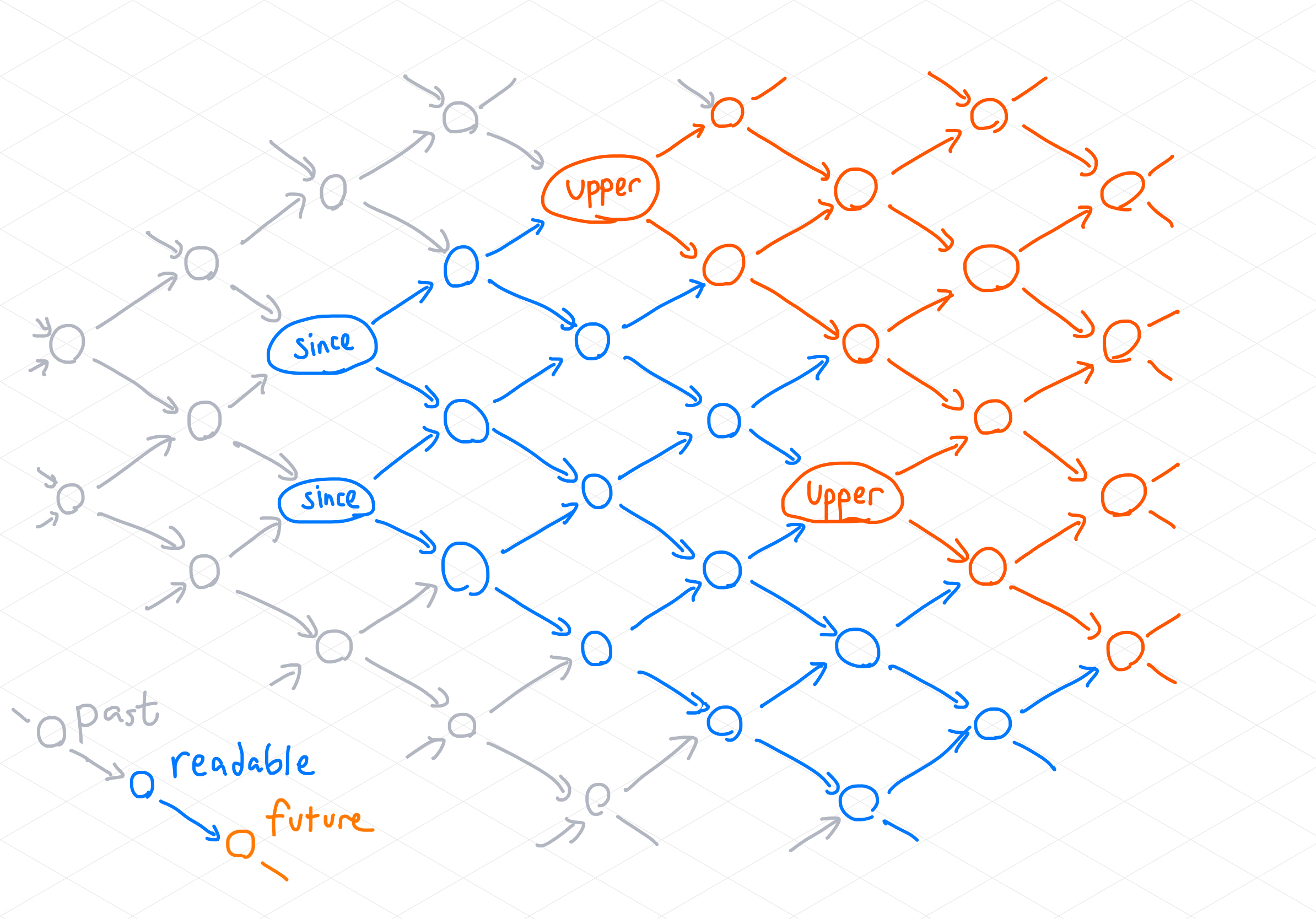
In this diagram, times are shown as a two-dimensional lattice forming a partial order; time generally flows left to right, and the precise order is shown by arrows. The since frontier is formed by two times labeled "since"; the upper frontier is formed by two times labeled "upper". Times later than upper are drawn in orange: these times are in the unknown future of the pTVC. Times not later than or equal to since are drawn in gray: these times are in the forgotten past. Only times in blue--those between since and upper--can be correctly read.

Update-set representations of TVCs and pTVCs

Because the set of times is in general very large, and because TVCs usually change incrementally, it is usually more efficient to represent a TVC as a set of updates which encode changes between collection versions. An update is a triple [data, time, diff]. The data specifies what element of the collection version is changing, the time gives the time the change took place, and the diff is the change in multiplicity for that element.

Given a collection version cv1 and an update u = [data, time, diff], we can apply u to cv1 to produce a new collection version cv2: apply(cv1, u) => cv2. cv2 is exactly cv1, but with multiplicity(cv2, data) = multiplicity(cv1, data) + diff.

We can also apply a countable set of updates to a collection version by applying each update in turn. We write this apply(collection, updates). Since apply is commutative, the order does not matter. In practice, these are computers: all sets are countable. (If you're wondering about uncountable sets, the Möbius inversion might be helpful.)

Given a time t and two collection versions cv1 and cv2, we can find their difference: a minimal set of updates which, when applied to cv1, yields cv2.

diff(t, cv1, cv2) = { u = [data, t, diff] |
                      (data in cv1 or data in cv2) and
                      (diff = multiplicity(cv2, data) - multiplicity(cv1, data)) and
                      (diff != 0)
                    }

Isomorphism between update and time-function representations

Imagine we have a TVC represented as a set of updates, and wish to read the collection version at time t. We can do this by applying all updates which occurred before or at t to the empty collection version. This lets us go from an update-set representation to a time-function representation.

read(updates, t) =
  apply(cv0, { u = [data, time, diff] | u in updates and time <=t t })

Similarly, given a time-function representation tvc, we can obtain an update-set representation by considering each point in time and finding the difference between the version at that time and the sum of all updates from all prior times. If we take Materialize times as the natural numbers, this is simple: the update set for a given time t is simply the difference between the version at t-1 and the version at t.

updates(tvc, t) = diff(t, read(tvc, t - 1), read(tvc, t))

In general times may be partially ordered, which means there might be multiple prior times; there is no single diff. Instead, we must sum the updates from all prior times, and diff that sum with the collection version at t:

updates(tvc, t) = diff(t,
                       apply(cv0, prior-updates(tvc, t)),
                       read(tvc, t))

The updates prior to t are simply the union of the updates for all times prior to t:

prior-updates(tvc, t) = ⋃ updates(tvc, prior-t) for all prior-t <t t

These mutually-recursive relations bottom out in the initial time t0, and the corresponding initial collection version read(tvc, t0):

prior-updates(tvc, t0) = diff(t0, cv0, read(tvc, t0))

Using these definitions, we can inductively transform an entire time-function representation tvc into a set of updates for all times by taking the union over all times:

updates(tvc) = ⋃ updates(tvc, t) for all t in T

Update representation of pTVCs

We have argued that the time-function and update-set representations of a TVC are equivalent. Similarly, we can also represent a pTVC as a timeline, a set of updates, and the since and upper frontiers: ptvc = [timeline, updates, since, upper]. To convert between time-function and update-set representations of pTVCs, we use the same definitions we gave for TVCs above. This gives the following four-fold structure:

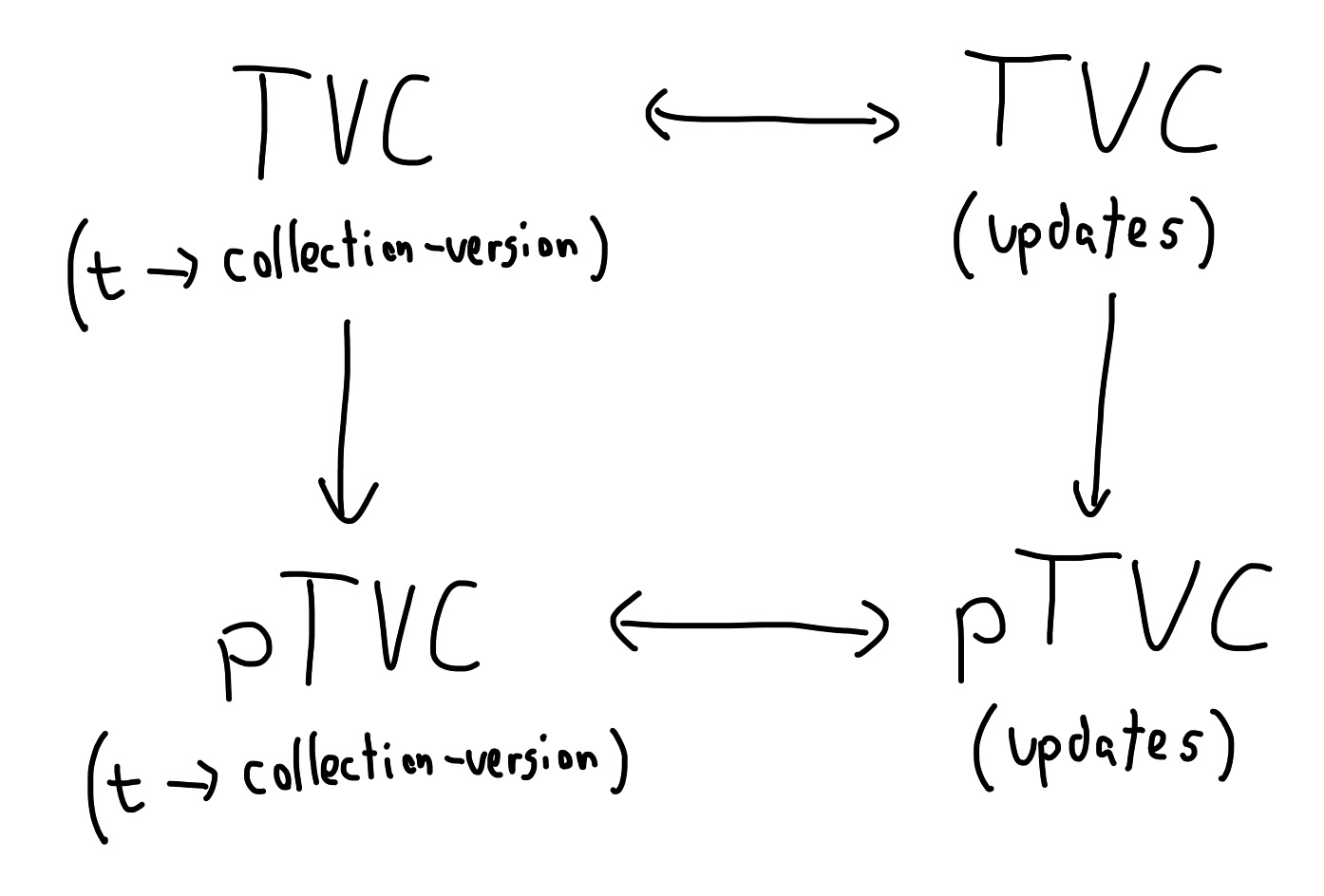
Materialize's goal is to physically store only the update-set representation of a pTVC, and for that pTVC to be an accurate view into the time-function and update-set representations of the corresponding TVC. To do this, we need to ensure each update-set pTVC maintains the correctness invariant: read(ptvc, t) = read(tvc, t) so long as t is at least since and not later than upper.

First, consider the empty pTVC ptvc0 = [timeline, {}, {t0}, {t0}]. ptvc0 is trivially correct since there are no times not later than than the upper frontier {t0}.

Next we consider two ways a pTVC could evolve, and wave our hands frantically while claiming that each evolution preserves correctness. This is not an exhaustive proof--we do not discuss, for example, the question of a pTVC which contains incorrect updates later than its upper frontier. However, this sketch should give a rough feeling for how and why Materialize works.

pTVC append

Let ptvc = [timeline, ptvc-updates, since, upper] be a correct view of some TVC's updates tvc_updates. Now consider appending a window of new updates to this pTVC, and advancing upper to upper': ptvc' = append(ptvc, upper', new-updates).

Which new updates do we need to add? Precisely those whose times are equal to or later than upper, and also not equal to or later than upper'.

ptvc' = [timeline,
         ptvc-updates ⋃ { u = [data, time, diff] in tvc_updates |
                          (upper <=t time) and not ( upper' <=t time)}
         since,
         upper']

Is ptvc' correct? Because since is unchanged and its updates between since and upper are unchanged, it must still be correct for any t between since and upper. And since it now includes every TVC update between upper and upper', it must also be correct for those times as well: their prior-updates are identical, by induction to times which were correct in the original ptvc. ptvc' is therefore correct for all times between since and upper'.

This allows us to advance the upper frontier of a pTVC by appending new updates to it (so long as we have every update between upper and upper') and still preserve correctness.

pTVC compaction

Again, let ptvc = [timeline, ptvc-updates, since, upper] be a correct view of some TVC. Now consider compacting all updates prior to some frontier since', in such a way that the collection versions read at times later than or equal to since' remain unchanged, to preserve correctness. We write this ptvc' = compact(ptvc, since'):

updates' = compact(updates, since')
ptvc' = [timeline, updates', since', upper]

Which updates can we compact, and which other updates do we compact them with? Consider this lattice of times flowing left to right, with two times in its since frontier. The set of all times at or after since is drawn in blue. We have also chosen two updates: one outlined in green at the top of the illustration, and one outlined in pink at the bottom left. The times which descend from those updates are filled with green or pink, respectively.

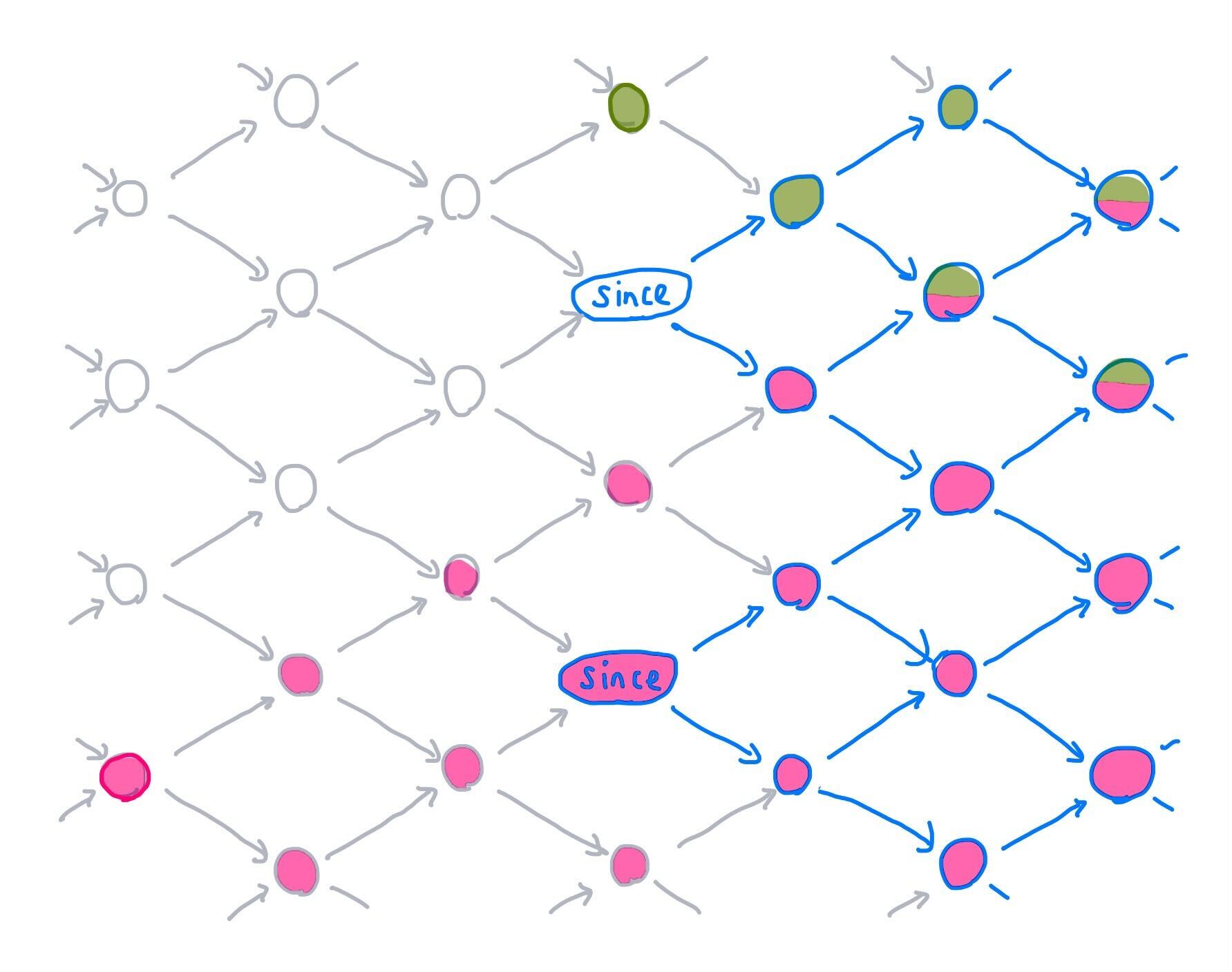
Now consider that each of these updates affects some times which are not at or after the since frontier. Since pTVC correctness does not require us to be able to read these times, we are free to "slide" each update around in any way that preserves the intersection of the update's downstream effects with the since region.

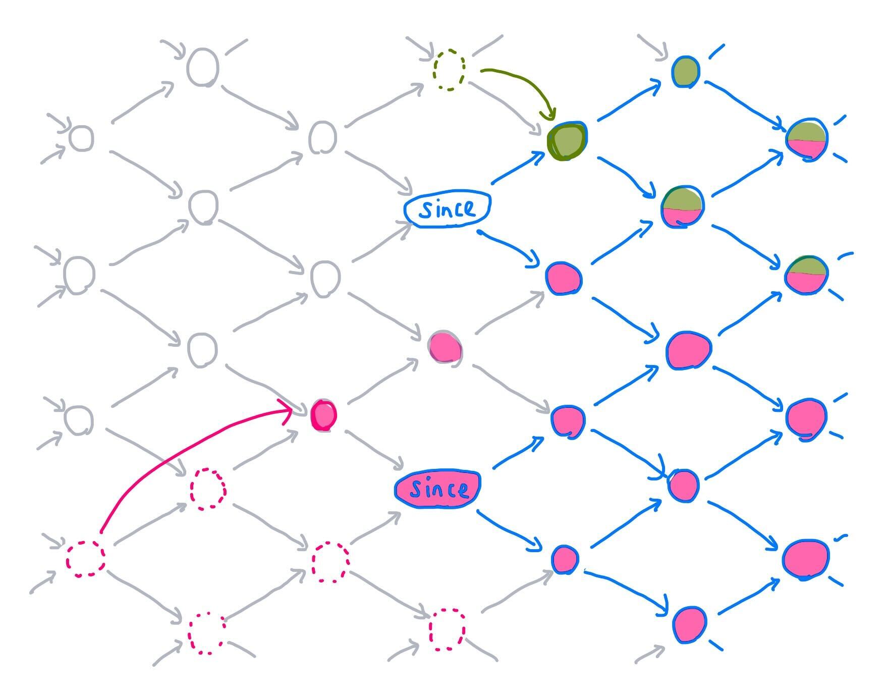
When sliding an update to a new time, which time is optimal? By "optimal", we mean the time which minimizes the number of downstream times which are not at or after since--in essence, how close can we slide an update at time t to the frontier since while preserving correctness? As Appendix A of the K-Pg SIGMOD paper shows, the answer is:

t' = meet (for all s in since) join(t, s)

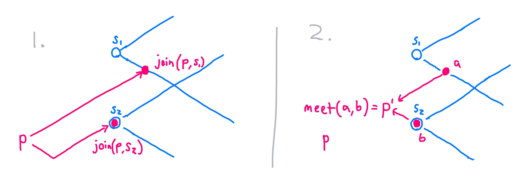
Given our two since frontier times of s1 and s2, we found the optimal time for the pink update at p by finding the first time where pink's effects intersected times at or after s1: join(p, s1); and did the same for s2. Then we projected backwards to the meet of those two times:

p' = meet(join(p, s1), join(p, s2))

Since join(t, s1) = t whenever t is at or after s1, this sliding process leaves any updates at or after since unchanged.

This transform allows us to slide updates forward from past times to new times, which reduces the number of distinct times in the updates set, but does not reduce the set's cardinality. However, we can take advantage of a second property for updates: given two updates u1 and u2 with the same data and time, and diffs diff1 and diff2 respectively, and any collection version c,

apply(c, {u1, u2}) = apply(c, [data, time, diff1 + diff2])

This allows us to fold updates to the same data together after sliding updates forward to the same time. Where diff1 + diff2 = 0, we can discard u1 and u2 altogether.

In summary: compact(ptvc, since') advances ptvc's since to since', slides some of ptvc's updates forward to new times (when doing so would not affect the computes states at or after since), and merges some those updates together by summing diffs for the same data and time. The resulting pTVC preserves correctness and likely requires fewer updates to store.

Time evolution of pTVCs

Materialize's goal is to keep track of a window of each relevant TVC over time. At any given moment a TVC is represented by a single ptvc = [updates, since, upper] triple. Each TVC begins with the empty ptvc0, which is a correct representation of every TVC. As new information about the TVC becomes available, Materialize appends those updates using append(ptvc, upper', new-updates). To reclaim storage space, Materialize compacts ptvcs using compact(ptvc, since'). Since both append and compact preserve pTVC correctness, Materialize always allows us to query a range of times (those between the current since and upper), and obtain the same results as would be observed in the "real" TVC.

During this process the since and upper frontiers never move backwards---and typically, they advance.

GlobalIds

A GlobalId is a globally unique identifier used in Materialize. One of the things Materialize can identify with a GlobalId is a TVC. Every GlobalId corresponds to at most one TVC. This invariant holds over all wall-clock time: GlobalIds are never re-bound to different TVCs.

There is no complete in-memory representation of a TVC in Materialize: such a thing would require perfect knowledge of the collection's versions over all time. Instead, we use GlobalIds to refer to TVCs.

The TVC Map

To track changing pTVCs over time, Materialize maintains a mutable TVC map. The keys in this map are GlobalIds, and the values are pTVCs. Each GlobalId in the TVC map identifies a single logical TVC, and the pTVC that ID refers to at any point in wall-clock time corresponds to that TVC. In short, the TVC map allows one to ask "What is the current pTVC view of the TVC identified by GlobalId gid?

The life cycle of each GlobalId follows several steps:

The GlobalId is initially not yet bound.

In this state, the GlobalId cannot be used in queries, as we do not yet know what its initial since will be.
The GlobalId is bound to some definition with an initially equal since and upper (e.g. ptvc0).

The partial TVC can now be used in queries, those reading from since onward, though results may not be immediately available. The collection is initially not useful, as it will not be able to immediately respond about any time greater or equal to since but not greater or equal to upper. However, the initial value of since indicates that one should expect the data to eventually become available for each time greater or equal to since.
Repeatedly, either of the these two steps occur:

a. The upper frontier advances, revealing more of the future of the pTVC.

b. The since frontier advances, concealing some of the past of the pTVC.
Eventually, the upper frontier advances to the empty set of times, rendering the TVC unwriteable.
Eventually, the since frontier advances to the empty set of times, rendering the TVC unreadable.

The GlobalId is never reused.

Architecture

We've sketched a formal model for how to represent time-varying collections as update-set pTVCs, and how we keep track of the current state of those pTVCs while appending new records to and compacting old records within them. We next discuss where and how in Materialize these pTVCs are stored, where updates come from, and how users query them.

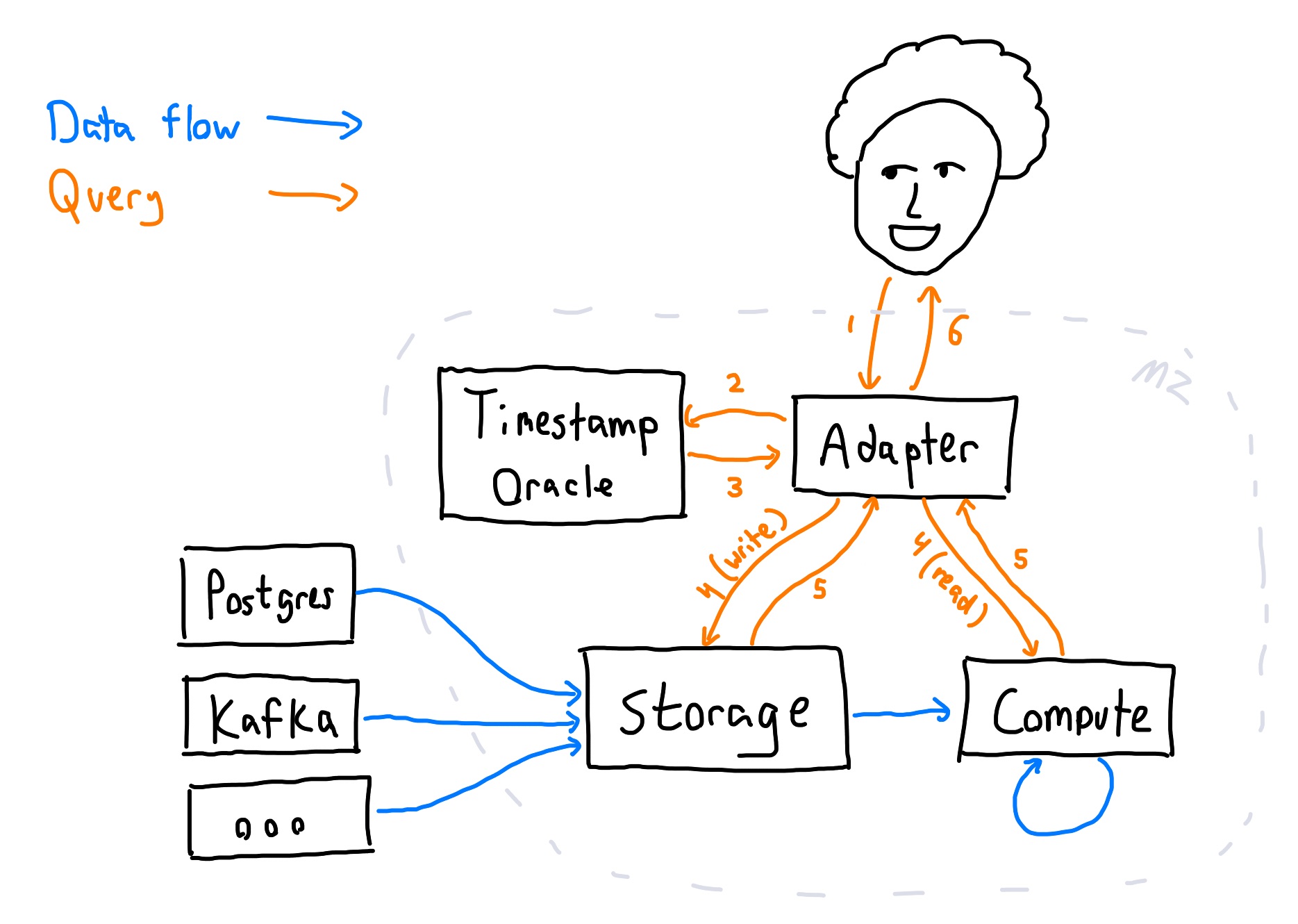
Updates flow into Materialize from external systems like Postgres and Kafka. They arrive first at the storage subsystem, which stores raw update triples for pTVCs. From there, they percolate through the compute subsystem, which uses differential dataflow to maintain materialized views. Each of these views is also a pTVC. Storage and compute cooperate to ensure pTVC correctness always holds.

Users query Materialize using SQL. That SQL is interpreted by an adapter, which transforms SQL queries into updates, reads, or creation of specific TVCs at specific times. Those times (where not explicitly specified) are chosen by a timestamp oracle. The adapter sends writes to storage, and reads values from compute.

Storage and Compute

Materialize produces and maintains bindings of GlobalIds to time-varying collections in two distinct ways:

The Storage layer records explicit TVCs in response to direct instruction (e.g. user DML), integrations with external sources of data, and feedback from Materialize itself. The representation in the Storage layer is as explicit update triples and maintained since and upper frontiers. The primary property of the Storage layer is that, even across failures, it is able to reproduce all updates for times that lie between since and upper frontiers that it has advertised.
The Compute layer uses a view definition to transform (possibly multiple) input TVCs into a new output TVC. The output TVC varies exactly with the input TVCs: For each time, the output collection at time equals the view applied to the input collections at time. We call this process of maintaining an output TVC that varies with input TVCs a dataflow.

The Storage and Compute layers both manage the since and upper frontiers for the GlobalIds they manage. For both layers, the since frontier is controlled by their users and it does not advance unless it is allowed. The upper frontier in Storage is advanced when it has sealed a frontier and made the data up to that point durable. The upper frontier in Compute is advanced when its inputs have advanced and its computation has pushed updates fully through the view definitions.

Capabilities

The since and upper frontiers are allowed to advance through the use of "capabilities". Layers keep track of the capabilities they've issued, and use those capabilities to determine when frontiers may advance. Each capability names a GlobalId and a frontier.

ReadCapability(id, frontier) prevents the since frontier associated with id from advancing beyond frontier.
WriteCapability(id, frontier) prevents the upper frontier associated with id from advancing beyond frontier.

A capability presents the id and frontier values, but is identified by a system-assigned unique identifier. Any user presenting this identifier has the associated capability to read from or write to the associated pTVC. Actions which read or write will validate the capability (e.g. in case a lease has expired) and may return errors if the capability is not valid as stated.

Capabilities are durable, and their state is tracked by the system who associates a unique identifier with each. Capabilities can be cloned and transfered to others, providing the same rights (and responsibilities). Capabilities can be downgraded to frontiers that are greater or equal to the held frontier, which may then allow the since or upper frontier to advance. Capabilities can be dropped, which releases the constraint on the frontier, and the whichever ability (read or write) the capability provided. These actions are mediated by the system, and take effect only when the system confirms the action. Users can defer and batch these actions, modulo lease timeouts, imposing only on the freshness and efficiency of the system.

Capabilities may expire, as a lease, which may result in errors from attempts to exercise the capability.

It is very common for users to immediately drop capabilities if they do not require the ability. The write capability for most TVCs is dropped immediately (by the system) unless it is meant to be written to by users (e.g. a TABLE). The read capability may be dropped immediately if the user does not presently need to read the data. Capabilities may be recovered by the best-effort command AcquireCapabilities(id) to be discussed.

Storage

The Storage layer presents a narrow API about which it makes guarantees. It likely has a more verbose diagnostic API that describes its state, which should be a view over the results of these commands.

Create(id, description) -> (ReadCapability, WriteCapability): binds to id the TVC described by description.

The command returns capabilities naming id, with frontiers set to initial values chosen by the Storage layer.

The collection associated with id is based on description, but it is up to the Storage layer to determine what the source's contents will be. A standarad example is a Kafka topic, whose contents are "added" to the underlying collection as they are observed. The Storage layer only needs to ensure that it can reliably produce the updates between since and upper, and otherwise the nature of the content is up for discussion. It is an error to re-use a previously used id.
SubscribeAt(ReadCapability(id, frontier)): returns a snapshot of id at frontier, followed by an ongoing stream of subsequent updates.

This command returns the contents of id as of frontier once they are known, and updates thereafter once they are known. The snapshot and stream contain in-line statements of the subscription's upper frontier: those times for which updates may still arrive. The subscription will produce exactly correct results: the snapshot is the TVCs contents at frontier, and all subsequent updates occur at exactly their indicated time. This call may block, or not be promptly responded to, if frontier is greater or equal to the current upper of id. The subscription can be canceled by either endpoint, and the recipient should only downgrade their read capability when they are certain they have all data through the frontier they would downgrade to.

A subscription can be constructed with additional arguments that change how the data is returned to the user. For example, the user may ask to not receive the initial snapshot, rather that receive and then discard it. For example, the user may provide filtering and projection that can be applied before the data are transmitted.
CloneCapability(Capability) -> Capability': creates an independent copy of the given capability, with the same id and frontier.
DowngradeCapability(Capability, frontier'): downgrades the given capability to frontier', leaving its id unchanged.

Every time in the new frontier' must be greater than or equal to the current frontier.
DropCapability(Capability): downgrades a capability to the final frontier {}, rendering it useless.
Append(WriteCapability(id, frontier), updates, new_frontier): applies updates to id and downgrades frontier to new_frontier.

All times in updates must be greater or equal to frontier and not greater or equal to new_frontier.

It is probably an error to call this with new_frontier equal to frontier, as it would mean updates must be empty. This is the analog of the INSERT statement, though updates are signed and general enough to support DELETE and UPDATE at the same time.
AcquireCapabilities(id) -> (ReadCapability, WriteCapability): provides capabilities for id at its current since and upper frontiers.

This method is a best-effort attempt to regain control of the frontiers of a collection. Its most common uses are to recover capabilities that have expired (leases) or to attempt to read a TVC that one did not create (or otherwise receive capabilities for). If the frontiers have been fully released by all other parties, this call may result in capabilities with empty frontiers (which are useless).

The Storage layer provides its output through SubscribeAt and AcquireCapabilities, which reveal the contents and frontiers of the TVC. All commands are durable upon the return of the invocation.

Compute

The Compute layer presents one additional API command. The layer also intercepts commands for identifiers it introduces.

MaintainView([ReadCapabilities], view, [WriteCapabilities]) -> [ReadCapabilities]: installs a view maintenance computation described by view.

Each view is described by a set of input read capabilities, identifying collections and a common frontier. The view itself describes a computation that produces a number of outputs collections. Optional write capabilities allow the maintained view to be written back to Storage. The method returns read capabilities for each of its outputs.

The Compute layer retains the read capabilities it has been offered, and only downgrades them as it is certain they are not needed. For example, the Compute layer will not downgrade its input read capabalities past the since of its outputs.

The outputs of a dataflow may or may not make their way to durable TVCs in the Storage layer. All commands are durable upon return of the invocation.

Constraints

A view introduces constraints on the capabilities and frontiers of its input and output identifiers.

The view holds a write capability for each output that does not advance beyond the input write capabilities.

This prevents the output from announcing it is complete through times for which the input may still change. The output write capabilities are advanced through timely dataflow, which tracks outstanding work and can confirm completeness.
The view holds a read capability for each input that does not advance beyond the output read capabilities.

This prevents the compaction of inputs updates into a state that prevents recovery of the outputs. Outputs may need to be recovered in the case of failure, but also in other less dramatic query migration scenarios.

These constraints are effected using the capability abstractions. The Compute layer acquires and maintains read capabilities for collections managed by it, and by the Storage layer.

Adapter

The adapter layer translates SQL statements into commands for the Storage and Compute layers.

The most significant differences between SQL statements and commands to the Storage and Compute layers are:

The absence of explicit timestamps in SQL statements.

A SELECT statement does not indicate when it should be run, or against which version of its input data. The Adapter layer introduces timestamps to these commands, in a way that provides the appearance of sequential execution.
The use of user-defined and reused names in SQL statements rather than GlobalId identifiers.

SQL statements reference user-assigned names that may be rebound over time. The meaning, and even the validity, of a query depends on the current association of user-defined name to GlobalId. The Adapter layer maintains a map from user-assigned names to GlobalId identifiers, and introduces new ones as appropriate.

Generally, SQL is "more ambiguous" than the Storage and Compute layers, and the Adapter layer must resolve that ambiguity.

The SQL commands are a mix of DDL (data definition language) and DML (data manipulation language). In Materialize today, the DML commands are timestamped, and the DDL commands are largely not (although their creation of GlobalId identifiers is essentially sequential). That DDL commands are not timestamped in the same sense as a pTVC is a known potential source of apparent consistency issues. While it may be beneficial to think of Adapter's state as a pTVC, changes to its state are not meant to cascade through established views definitions.

Commands acknowledged by the Adapter layer to a user are durably recorded in a total order. Any user can rely on all future behavior of the system reflecting any acknowledged command.

Timestamp Oracle

The adapter assigns timestamps to DML commands using a timestamp oracle. The timestamp oracle is a stateful, linearizable object which (at a high gloss) provides a simple API:

AssignTimestamp(command) -> timestamp

Since the timestamp oracle is linearizable, all calls to AssignTimestamp appear to take place in a total order at some point between the invocation and completion of the call to AssignTimestamp. Along the linearization order, returned timestamps satisfy several laws:

The timestamps never decrease.
The timestamps of INSERT/UPDATE/DELETE statements are strictly greater than those of preceding SELECT statements.
The timestamps of SELECT statements are greater than or equal to the read capabilities of their input collections.
The timestamps of INSERT/UPDATE/DELETE statements are greater than or equal to the write capabilities of their target collection.

The timestamps from the timestamp oracle do not need to strictly increase, and any events that have the same timestamp are concurrent. Concurrent events (at the same timestamp) first modify collections and then read collections. All writes at a timestamp are visible to all reads at the same timestamp.

Some DML operations, like UPDATE and DELETE, require a read-write transaction which prevents other writes from intervening. In these and other non-trivial cases, we rely on the total order of timestamps to provide the apparent total order of system execution.

Several commands support an optional AS OF <time> clause, which instructs the Adapter to use a specific query time, if valid. If this clause is present, the adapter will not ask the timestamp oracle for a timestamp. The command will observe all writes up through time (if it reads) and be visible by all reads from time onward (if it writes).

Sources

Materialize supports a CREATE SOURCE command that binds to a user-specified name a GlobalId produced by the Storage layer in response to a Create command. A created source has an initial read capability and write capability, which may not be at the beginning of time. Two sources created with the same arguments are not guaranteed to have the same contents at the same time (said differently: Materialize uses nominal rather than structural equivalence for sources).

Sources remain active until a DROP SOURCE command is received, at which point the Adapter layer drops its read capability.

One common specialization of source is the "table". The CREATE TABLE command introduces a new source that is not automatically populated by an external source, and is instead populated by Append commands. The Adapter layer may use a write-ahead log to durably coalesce multiple writes at the same timestamp, as the Append command does not otherwise allow this. The DROP TABLE command drops both the read and write capabilities for the source.

Indexes

Materialize supports a CREATE INDEX command that results in a dataflow that computes and maintains the contents of the index's subject, in indexed representation. The CREATE INDEX command can be applied to any collection whose definition avoids certain non-deterministic functions (e.g. now(), rand(), environment variables).

Materialize's main feature is that for any indexable view, one receives identical results whether re-evaluating the view from scratch or reading it from a created index.

The CREATE INDEX command results in a MaintainView command for the Compute layer. The inputs to that command are GlobalId identifiers naming Storage or Compute collections. The command is issued with read capabilities all advanced to a common frontier (often: the maximum frontier of read capabilities in the input). The command returns a read capability for the indexed collection, which the Adapter layer maintains and perhaps regularly downgrades, as is its wont. The dataflow remains active until a corresponding DROP INDEX command is received by the Adapter layer, which discards its read capability for the indexed collection.

Transactions

The Adapter layer provides interactive transactions through the BEGIN, COMMIT, and ROLLBACK commands. There are various restrictions on these transactions, primarily because the Storage and Compute layers require you to durably write before you can read from them. This makes write-then-read transactions challenging to perform efficiently, and they are not currently supported. Read-only transactions are implemented by performing all reads at a single timestamp. Write-only transactions are implemented by buffering all writes and then applying them during commit at a single timestamp. Read-then-write transactions are implemented by performing all reads at some timestamp greater than or equal to all previous timestamps and then writing at a strictly later timestamp. Read-then-write transactions are implemented by performing all reads at some timestamp greater than or equal to all previous timestamps and then writing at a strictly later timestamp. Read-then-write transactions are only considered valid and applied if there are no updates to the query inputs at a time greater than the read timestamp and not greater than the write timestamp. Read-then-write transactions are ordered using the write timestamp in the total order of all transactions.

It is possible that multiple read-then-write transactions on disjoint collections could be made concurrent, but the technical requirements are open at the moment.

Read-after-write, and general transactions are technically possible using advanced timestamps that allow for Adapter-private further resolution. All MZ collections support compensating update actions, and one can tentatively deploy updates and eventually potentially retract them, as long as others are unable to observe violations of atomicity. Further detail available upon request.

It is critical that Adapter not deploy Append commands to Storage and Compute until a transaction has committed. These lower layers should provide similar "transactional" interfaces that validate tentative commands and ensure they can be committed without errors.

Compaction

As Materialize runs, the Adapter may see fit to "allow compaction" of collections Materialize maintains. It does so by downgrading its held read capabilities for the collection (identifier by GlobalId). Downgraded capabilities restrict the ability of Adapter to form commands to Storage and Compute, and may force the timestamp oracle's timestamps forward or delay a query response.

formalism.md 42 KB Permalink History Raw